❌

Reading view

Not All Black Holes Who Wander Are Lost
interacting galaxies Arp 147

Editor’s Note: Astrobites is a graduate-student-run organization that digests astrophysical literature for undergraduate students. As part of the partnership between the AAS and astrobites, we occasionally repost astrobites content here at AAS Nova. We hope you enjoy this post from astrobites; the original can be viewed at astrobites.org.

Title: Tracing Black Hole and Galaxy Growth Across Environments Since Cosmic Noon
Authors: Emma Jane Weller et al.
First Author’s Institution: Yale University
Status: Published in ApJ

They say you can’t choose your hometown, but it still ends up shaping who you become. Turns out the same is true for black holes. The galaxy a black hole grows up in will have a major impact on how it will live out the rest of its life. Similarly, the black hole can leave a lasting impression on its galaxy!

Astronomers have long known that a galaxy’s stellar mass (the combined mass of all its stars) tracks pretty tightly with the mass of the black hole sitting at its centre: bigger galaxy, bigger black hole. This is one pillar of the idea that galaxies and their central black holes coevolve; that is, their life stories are tangled up with one another from early on. But ever since JWST started spotting suspiciously large black holes in the early universe, astronomers have been debating whether this relationship holds steady across cosmic time, or whether the rules were different when the universe and everything in it was younger.

Not Everyone Stays in the Town Centre

Most previous studies of the relationship between black holes and their galaxies have focused only on the central black hole: the biggest, most famous resident of a galaxy, sitting right downtown at its centre. That’s a reasonable place to start, since the central black hole is usually the most massive one around and tends to dominate the story. But this article’s authors wanted to know what happens to everyone else in town, too!

That includes satellite black holes, which are the central black holes of smaller “satellite” galaxies that orbit a bigger “primary” galaxy, a bit like a small town around a big city. It also includes a stranger, more recently discovered population: wandering black holes. These are the black hole equivalent of someone whose hometown got swallowed up by an expanding metropolis, and who never quite settled into their new surroundings.

Here’s how it happens: when a small satellite galaxy merges with a larger one, the satellite gets torn apart by tidal forces and its gas and stars are stripped away. However, its central black hole is often left behind, drifting through the new, much bigger galaxy on a wide orbit. The process that would normally drag a black hole down to the centre of a galaxy, called dynamical friction, is painfully slow, so wanderers can spend billions of years roaming the outskirts.

Two Cities, Two Sets of Rules

To study how these different black hole “life paths” shape, and are shaped by, their host galaxies, the authors turned to two cosmological simulations, ASTRID and TNG300, which handle black hole physics quite differently.

In TNG300, black holes are assumed to start fairly massive and are snapped straight to the centre of their host galaxy at every timestep. This makes mergers happen quickly and often, but it also means there’s no such thing as a wandering black hole in TNG300.

ASTRID, on the other hand, seeds smaller black holes and lets them move more realistically through their galaxy using a subgrid dynamical friction model. This is what allows wandering black holes, with their slow, aimless orbits, to exist and be studied in the first place.

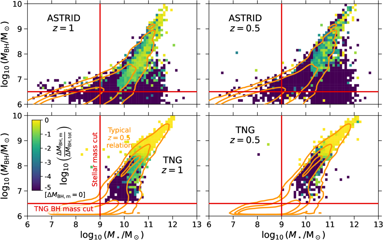
Figure 1 reveals a lot at once. First, ASTRID (the simulation that allows wandering black holes and tidally stripped satellites) has whole new neighbourhoods on the map that simply don’t exist in TNG300. Those populations clearly aren’t following the same tidy, linear coevolution that central black holes enjoy with their galaxies. Second, the most massive black holes tend to be the most yellow, meaning mergers did the heavy lifting for their growth. This is especially pronounced in TNG300, where roughly 80–90% of the growth of the most massive black holes comes from mergers. Meanwhile, the wanderers and stripped satellites sit at the deep-purple end: these black holes have barely merged with anyone at all.
relation between black hole mass and host galaxy stellar mass

Figure 1: How black hole mass relates to host galaxy stellar mass, shown at two snapshots in cosmic history, 8 and 5 billion years ago, for both simulations (ASTRID: top row; TNG300: bottom row). Colour shows what fraction of each black hole’s growth since the last snapshot came from mergers, from purple (grown almost entirely by slowly swallowing gas) to yellow (grown mostly by swallowing other black holes). [Weller et al. 2026]

Four Kinds of Black Hole Life Stories

Pulling all of this together, the authors sketch out a kind of “neighborhood map” of black hole fates, sorted by where a black hole ends up on the mass-relation plot and how it got there (see Figure 2).
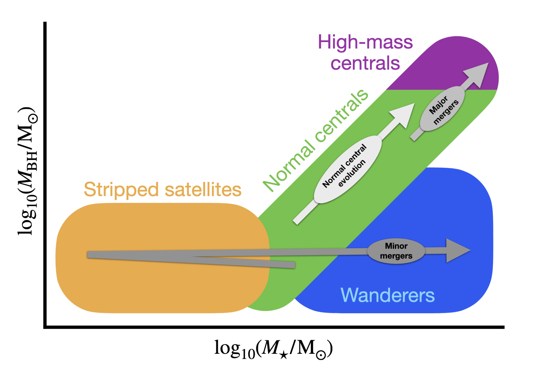
diagram showing the distinct populations revealed by the black hole mass–stellar mass relation

Figure 2: The distinct black hole populations revealed by the black hole mass–stellar mass relation, and the evolutionary path that lands each population in its corner of the map. [Weller et al. 2026]

  • Normal centrals are the homebodies. They sit at the centre of primary or satellite galaxies and grow up steadily alongside their hometown, climbing the mass relation together through a healthy mix of accretion and the occasional merger. Their galaxies keep forming stars the whole time in a functional, unremarkable, thoroughly nice place to live.
  • High-mass centrals are the ones who “made it.” These are central black holes in big primary galaxies, and their growth comes overwhelmingly from mergers with other black holes. Once they get big enough, they start throwing their weight around: their jets blast gas out of the galaxy, shutting down both star formation and their own further growth.
  • Stripped satellites are the annexed suburbs. They start out on the normal mass relation, but a merger with a bigger galaxy tears away their gas and stars, shrinking their stellar mass while their black hole is left comparatively overweight for its new, smaller home. With their gas reserves gone, star formation grinds to a halt, and their black holes, starved of fuel, barely grow either.
  • Wanderers are the ones who moved to the big city and never quite settled in. They start out on the normal relation inside a satellite galaxy, but when that galaxy merges into something much bigger, they’re left drifting through unfamiliar, low-density territory. With little gas around to feed on and almost no chance of merging with anyone else, their growth basically stalls.

This four-way map is a genuinely useful new way to read the black hole–galaxy relation: a black hole’s exact position on the plot isn’t just a number, it’s a fossil record of everywhere it’s ever “lived.”

There’s plenty more in the article we haven’t covered here, including how quenching plays out over time, how these results stack up against the local universe, and a closer look at how star formation rates and black hole accretion rates track each other across all four populations. If any of this piqued your interest, the full article is well worth a read.

Original astrobite edited by Ryan White and Chloe Klare.

About the author, Jayde Willingham:

I am a first-year PhD student at Swinburne University of Technology studying the early universe and how the first galaxies came to be. My work combines observations and theoretical modelling to explore how galaxies form, evolve, and shape the universe we see today. When I’m not at my desk or doing SciComm, I’m probably reading a good book with a hot beverage under a cozy blanket.

The post Not All Black Holes Who Wander Are Lost appeared first on AAS Nova.
  •  

The Invisible Architecture Between the Stars

NGC 2467

Editor’s Note: Astrobites is a graduate-student-run organization that digests astrophysical literature for undergraduate students. As part of the partnership between the AAS and astrobites, we occasionally repost astrobites content here at AAS Nova. We hope you enjoy this post from astrobites; the original can be viewed at astrobites.org.

Title: Phase-Dependent Magnetic Coherence in the Turbulent Interstellar Medium
Authors: Iryna S. Butsky et al.
First Author’s Institution: Stanford University
Status: Accepted to ApJ

The space between stars isn’t empty, because it’s threaded with magnetic fields that shape how gas moves and steer cosmic rays as they race across the galaxy. As a result, understanding how the magnetic field is structured within different components of the interstellar medium, specifically clouds of different temperatures, is a key part of understanding how the interstellar medium we see today takes shape.

Because magnetic fields are invisible, astronomers need tracers to reveal their structure. One such tracer is the emission from dust grains. Dust grains are not spherical, and a dust grain’s long axis tends to align at a right angle to the magnetic field, causing dust grains to emit light that vibrates in a particular direction. This is called polarized emission. If the magnetic field in a region is very ordered, the grains all align the same way, and a large fraction of their emitted light vibrates in the same direction, giving a high polarization fraction. This fraction is therefore used as a proxy for whether the field can maintain a consistent direction on large scales (an ordered/regular magnetic field).

Comparing the polarization fraction with other tracers of gas lets astronomers infer the field’s structure in the interstellar medium. Previous observations found that the polarization fraction correlates with the fraction of cold gas, but not with the total amount of gas along the line of sight. This suggests that the field is preferentially ordered within cold clouds rather than warm clouds. Curiously, this seemed to contradict other studies that found the field to be more ordered in the warm clouds. Such disagreements are where simulations become useful: because the true magnetic field is known in a simulation, astronomers can test which interpretation the observations actually support.

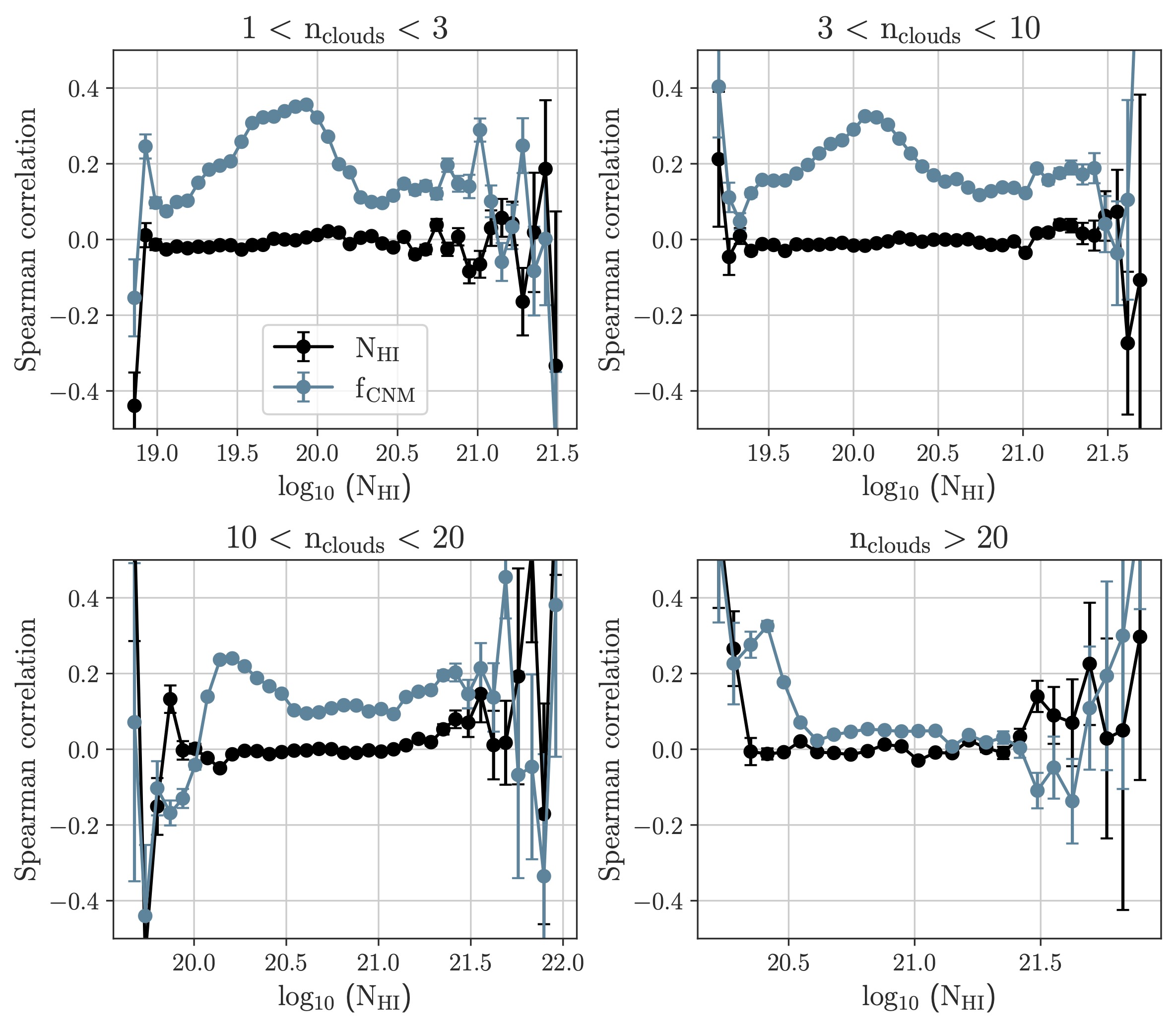
In this article, the authors use high-resolution numerical simulations to reproduce the relationship between polarization fraction and cold cloud fraction. They find that as long as the line of sight crosses fewer than about 20 clouds, the polarization fraction correlates with the cold cloud fraction, but not with the total neutral gas (Figure 1). This matches earlier observations, where the correlation shows up at high galactic latitudes, which point out of the galactic plane and therefore cross only a few cold structures. When too many clouds lie along the line of sight, each cloud carries an ordered field pointing in a different direction. Averaged together, these vibration directions cancel out, lowering the polarization fraction and washing the correlation away.

Plots showing the correlation between dust polarization fraction, the total gas amount, and the fraction of cold medium along the line of sight

Figure 1: Correlation between dust polarization fraction, the total gas amount (neutral hydrogen column density, NHI), and the fraction of cold medium along the line of sight (fCNM) for projections of different path lengths. The polarization fraction correlates with fCNM but not with NHI. The correlation disappears once many clouds lie along the line of sight (see lower-right panel). [Butsky et al., in press]

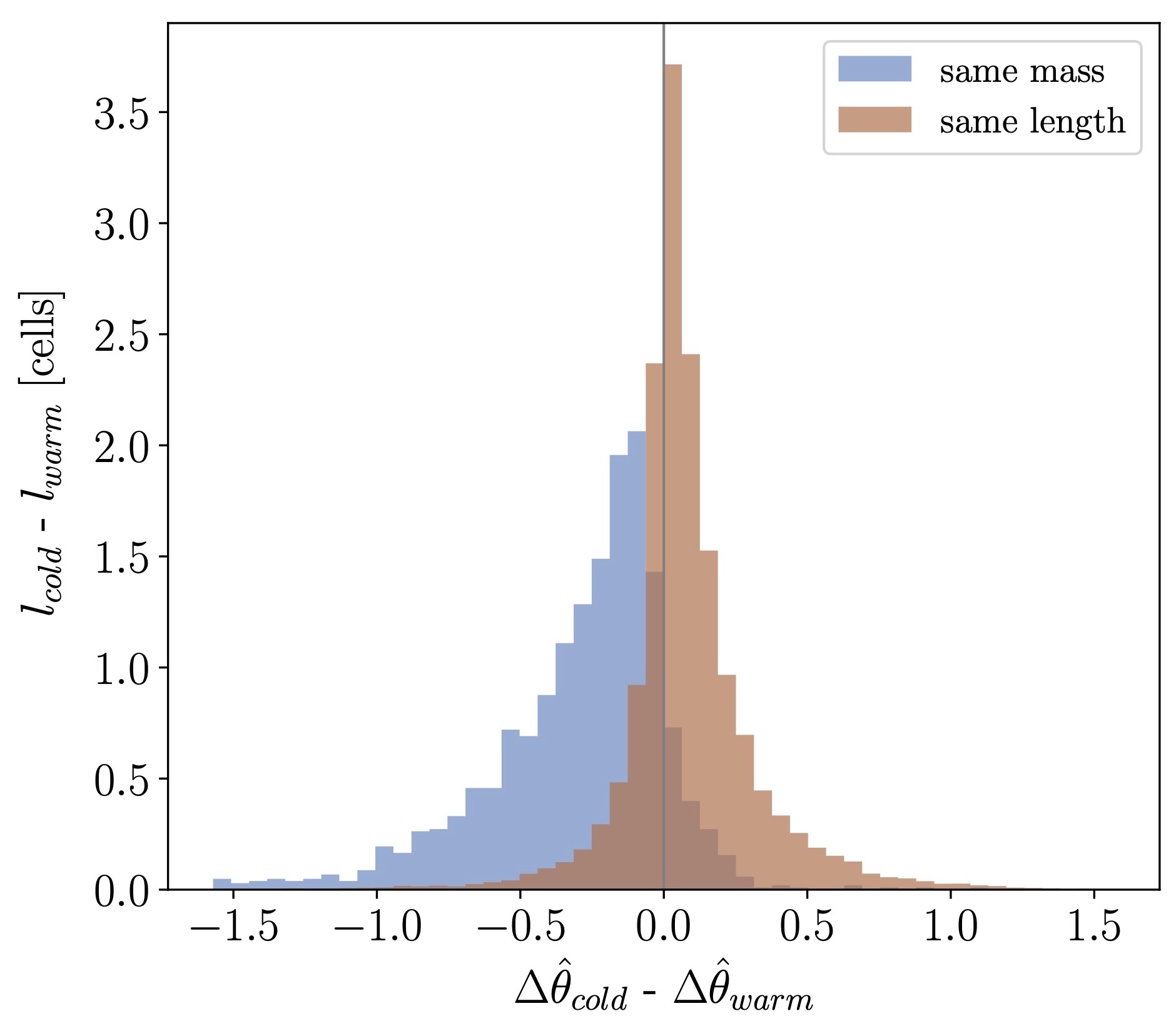
Distribution of the angle difference between the average magnetic field and the line of sight for cold and warm clouds

Figure 2: Distribution of the angle difference between the average magnetic field and the line of sight for cold and warm clouds, shown for clouds matched by mass and by length. A smaller angle difference means a more ordered field. At similar mass, cold clouds show a more ordered field; at similar length, the reverse holds. [Adapted from Butsky et al., in press]

Since the simulation reproduces the observational result, does it therefore agree with the conclusion that magnetic fields are genuinely more ordered in the cold neutral medium? The authors argue that the answer depends on how you measure “order.” Comparing the magnetic field direction in individual dense clouds, they find that cold clouds have more ordered fields when compared against warm clouds of similar mass, but the conclusion flips when comparing clouds of similar length (Figure 2).

This apparent paradox comes from the different nature of cold and warm clouds. Cold clouds are denser and more compact, occupying much smaller physical scales than warm clouds. So to match the length of a warm cloud, you have to string together several cold structures, sampling more of the field’s variation and making the cold gas look disordered. Measured per unit length, then, warm clouds appear more ordered. Measured per unit mass, cold clouds appear more ordered. Crucially, when we observe dust emission, we are naturally weighting by mass, so real observations effectively trace the polarization fraction per unit mass, the regime in which the cold clouds are the more coherent phase.

In the end, this work shows that the ordering of interstellar magnetic fields depends on both the gas phase and how we choose to measure it. Cold clouds carry more coherent fields per unit mass, which is exactly the quantity dust observations trace, resolving an apparent contradiction between earlier studies. It is a reminder that even our best observations come with hidden assumptions, and that simulations, where the true field is known, are essential for interpreting what the sky is really telling us.

Original astrobite edited by Viviana Cáceres.

About the author, Sandy Chiu:

I’m a PhD candidate at the University of Michigan, Ann Arbor. I’m interested in numerical simulations of cosmic rays feedback in galaxies and their comparison with observation.

The post The Invisible Architecture Between the Stars appeared first on AAS Nova.
  •  

SPHEREx: The Niftiest Space Telescope You May Not Have Heard Of

SPHEREx

Editor’s Note: Astrobites is a graduate-student-run organization that digests astrophysical literature for undergraduate students. As part of the partnership between the AAS and astrobites, we occasionally repost astrobites content here at AAS Nova. We hope you enjoy this post from astrobites; the original can be viewed at astrobites.org.

Title: The SPHEREx Satellite Mission
Authors: James J. Bock et al.
First Author’s Institution: California Institute of Technology; Jet Propulsion Laboratory
Status: Published in ApJ

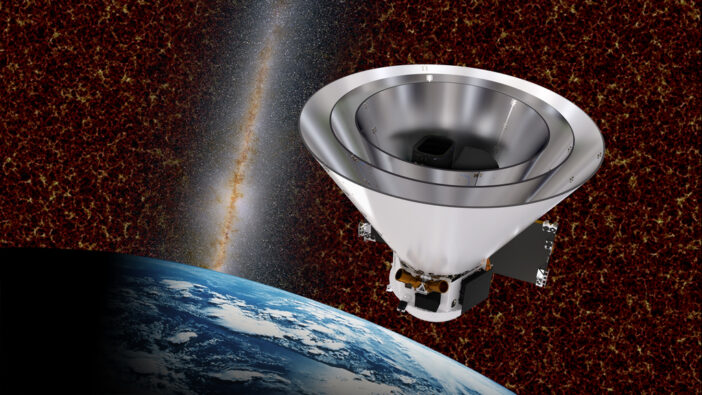
You know JWST. You’ve likely heard about the recently launched Nancy Grace Roman Space Telescope. But did you know that NASA launched a third space telescope focused on infrared astronomy just last year? That telescope, called SPHEREx (short for Spectro-Photometer for the History of the Universe, Epoch of Reionization, and Ices Explorer, but we’ll forgive the tortured acronym), is currently carrying out its ambitious mission to record an infrared spectrum for every point in the sky. Let’s break down SPHEREx’s three main science goals and then discuss how SPHEREx will accomplish its mission.

Goal #1: Stress-Testing Cosmic Inflation

According to our best current models of cosmology, the very early universe experienced a rapid burst of accelerating expansion called cosmic inflation. During inflation, small regions of the universe that by chance had slightly higher energy density than their neighbors (due to quantum fluctuations) expanded to huge scales. Because these regions were very gravitationally attractive, once inflation ended, they became the seeds where matter accumulated and eventually formed galaxies.

This means that the distribution of galaxies that we see today is a reflection of the properties of inflation (i.e., what the quantum fluctuations were like and how inflation supersized them). SPHEREx will assemble the largest atlas of galaxies ever, recording the three-dimensional positions of hundreds of millions of galaxies across the entire sky. To do this, SPHEREx must figure out how far away these galaxies are from Earth, using their redshifts. SPHEREx’s low-resolution infrared spectroscopy allows for moderately precise measurements of these redshifts. By performing statistical analyses of how galaxies are separated from each other, SPHEREx will test different theories of inflation, like whether inflation was driven by multiple fields.

Goal #2: Frozen Assets

Astronomers are racing to find evidence for life (or at least habitability) in the atmospheres of exoplanets through transmission spectroscopy. However, we don’t know for sure how molecules that could be used in biological processes (called biogenic molecules, these include water, carbon dioxide, carbon monoxide, and methanol) even end up on planets.

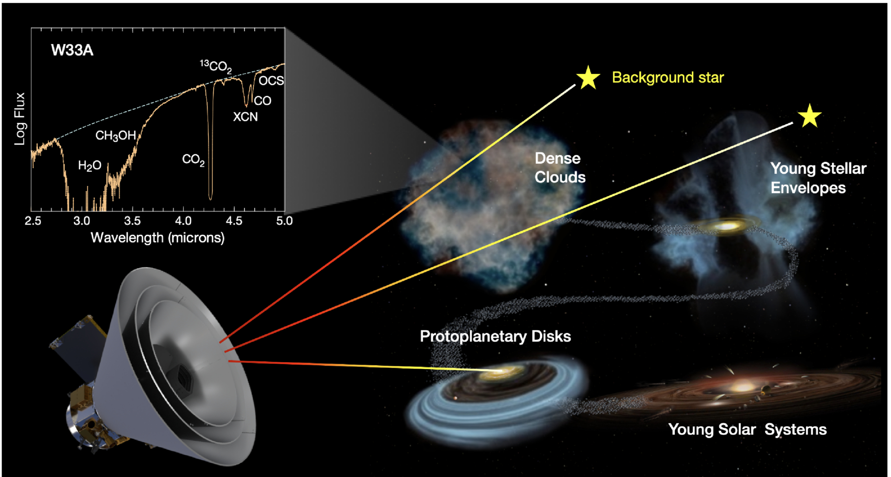
We think that a large fraction of these molecules are frozen onto dust grains throughout the interstellar medium. When a new star forms in the interstellar medium, this ice and dust would become part of the star’s protoplanetary disk. The ice species can help create planetesimals (which may grow into planets) or can later deliver biogenic molecules to planetary surfaces. Earth’s oceans likely came (at least in part) from collisions with icy asteroids. As Figure 1 shows, SPHEREx will measure the abundance of ice species in different environments that track the history of solar system formation, from dense clouds in the interstellar medium that may soon form stars to regions around newborn stars and evolving protoplanetary disks. In this way, SPHEREx will track how biogenic molecules from the interstellar medium can end up on planets.

cartoon showing the types of sources SPHEREx will target in its search for biogenic molecules

Figure 1: Examples of the sources SPHEREx will look at to search for biogenic ice species. In the top left, what the spectra of these sources will look like if those species are present: each type of ice leaves a distinct fingerprint in an infrared spectrum. [Bock et al. 2026]

Goal #3: Your Noise Is SPHEREx’s Signal

SPHEREx will measure an infrared spectrum for every point in the sky — even those that don’t contain galaxies or stars that we can resolve. These points are instead dominated by diffuse extragalactic background light. This light comes from many different sources, including stars, dust, and quasars, from the early universe to the present day, all added together incoherently. For most telescopes, the extragalactic background light is just a frustrating source of noise. For SPHEREx, it’s a treasure trove. We can compare the properties of the extragalactic background light that SPHEREx measures (its spectrum and how it fluctuates across the sky) to theoretical predictions and see if we seem to be missing anything. SPHEREx’s very broad infrared spectra — capturing redshifted light from the very early universe — and total sky coverage are crucial for this purpose. For instance, the SPHEREx team will try to isolate emission from the first stars and galaxies, which ionized most of the gas in the universe in the epoch of reionization. By understanding this and other contributions to the extragalactic background light, we can test hypotheses about how galaxies form and evolve.

Making It Happen

Beyond inflation, ices, and extragalactic background light, SPHEREx’s all-sky infrared spectra will be invaluable for countless other science cases, like studying asteroids, characterizing the atmospheres of stars that host exoplanets, and even understanding the upper atmosphere of Earth, through which SPHEREx orbits.

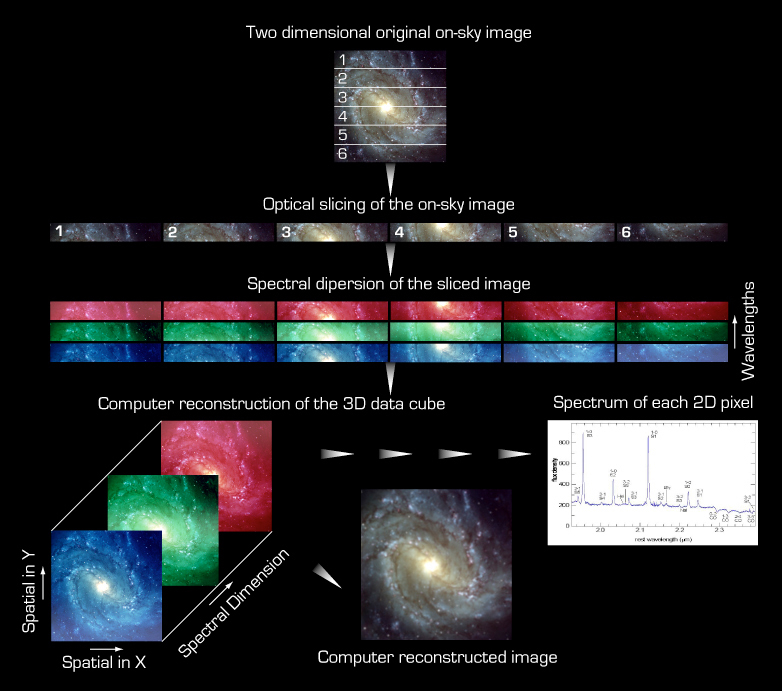
But how can SPHEREx even make a spectrum for every point in the sky? An image of some part of the sky is fundamentally two-dimensional, and measuring how the brightness of every point changes with wavelength adds a third dimension. Astronomers have come up with many ways to solve this problem. Integral field spectroscopy approaches typically involve splitting an image into small regions or strips, then using a dispersive element like a prism or grating to make a spectrum of each region, and finally putting these spectra side by side on a camera. Figure 2 shows an example of this strategy, as well as what the final three-dimensional “datacube” looks like after processing.

demonstration of integral field spectroscopy

Figure 2: A demonstration of the principle of integral field spectroscopy. [ESO; CC BY 4.0]

This approach is fairly complicated, relying on fancy optics, a prism or grating, and oftentimes optical fibers. From Figure 2, note that you could also make the final “datacube” product if you simply took many images with narrow filters that let through different wavelengths of light. This takes to an extreme the approach astronomers use for spectral energy distribution fitting. Of course, this would require an exorbitant number of filters. Here, the SPHEREx team had a stroke of genius: instead of having many different filters, what if you had a filter where the transmitted wavelength changes linearly across the filter? Each row would let through a different wavelength. To get a full spectrum for all points in an image, you could take many exposures, moving the telescope slightly between each exposure so points in the image fall on different rows each time.

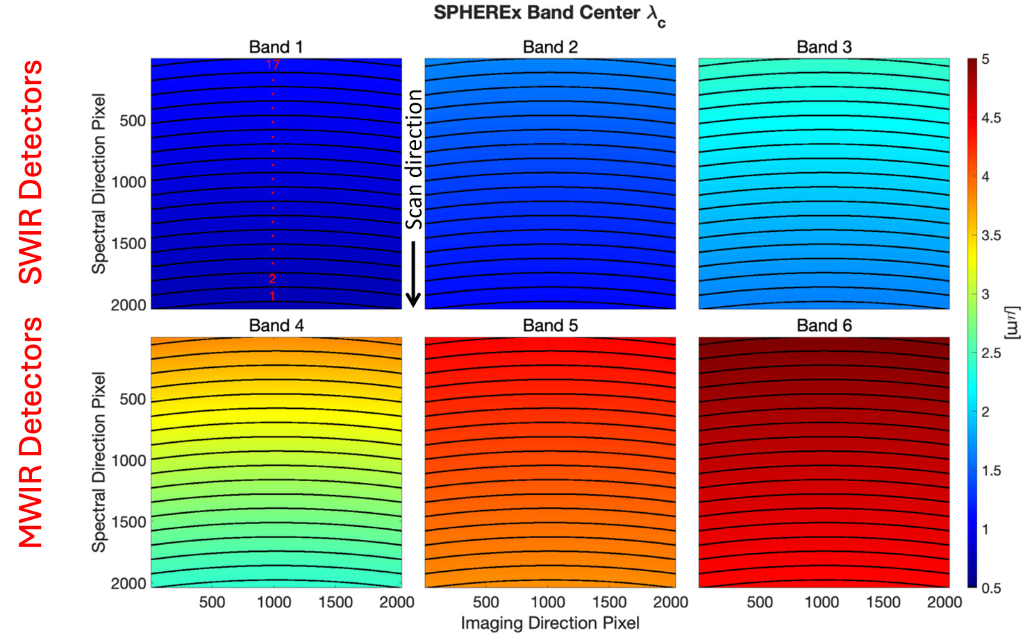
This is the SPHEREx survey strategy, with a few complications. First, before any filter, SPHEREx splits incoming light into two beams, with short-wave infrared light (SWIR, with 0.75 μm < λ < 2.42 μm) going in one direction and mid-wave infrared light (MWIR, 2.42 μm < λ < 5.00 μm) going in another. SPHEREx makes images with these two beams on different sets of detectors, so it can measure the brightness of an object at one SWIR wavelength and one MWIR wavelength simultaneously. The SPHEREx field of view covers 10.5° by 3.5°, with the SWIR and MWIR images each spread across three detectors. Every detector has a different linearly variable filter. To get a complete infrared spectrum of a given point in the sky, SPHEREx moves that point to 17 different positions on each detector. This requires 51 different telescope (17 × 3 detectors) pointings in all and yields 102 spectral values (51 × 2 for the SWIR and MWIR beams). Figure 3 shows the 17 bands on each of the six SPHEREx detectors, each corresponding to a different wavelength value.

plots showing the central wavelength of the spectral response of each pixel measured over the six detector arrays in the focal plane

Figure 3: The wavelength of light that each part of each SPHEREx detector is sensitive to. A point in the sky is imaged on one short-wave infrared detector (top row) and one mid-wave infrared detector (bottom row) simultaneously. SPHEREx measures each point in the sky at 102 different wavelengths by placing the point at 17 different positions on each of the detectors. [Adapted from Bock et al. 2026]

While it would take decades to collect spectra for every point on the sky with conventional methods for integral field spectroscopy, the SPHEREx team devised a nifty solution that will collect this dataset in a few years. Soon, SPHEREx will start answering questions about cosmic inflation, interstellar ices, and extragalactic background light, while its rich dataset will be relevant for decades to come. So tell all your friends about SPHEREx (even if you can’t remember what the acronym stands for)!

Original astrobite edited by Veronika Dornan.

About the author, Chris Layden:

Chris is a PhD candidate in astrophysics at the Massachusetts Institute of Technology. His primary research interest is developing instrumentation that enables high-speed astronomical observations. With such instruments, he studies the most rapidly varying phenomena in the sky, including millisecond pulsars, accreting black holes, and solar system objects whizzing past background stars. Outside of astronomy, Chris enjoys reading classic novels, playing ultimate frisbee, and hanging out with his wife and dog.

The post SPHEREx: The Niftiest Space Telescope You May Not Have Heard Of appeared first on AAS Nova.

  •  

An Early Discovery by Rubin Observatory

stars seen by Rubin Observatory

Editor’s Note: Astrobites is a graduate-student-run organization that digests astrophysical literature for undergraduate students. As part of the partnership between the AAS and astrobites, we occasionally repost astrobites content here at AAS Nova. We hope you enjoy this post from astrobites; the original can be viewed at astrobites.org.

Title: Discovery of the Distant, Ultra-Faint Milky Way Satellite Aquarius IV with the Vera C. Rubin Observatory Early Data Preview 2
Authors: William Cerny et al.
First Author’s Institution: Yale University
Status: Published in RNAAS

Warming Up the World’s Largest Camera

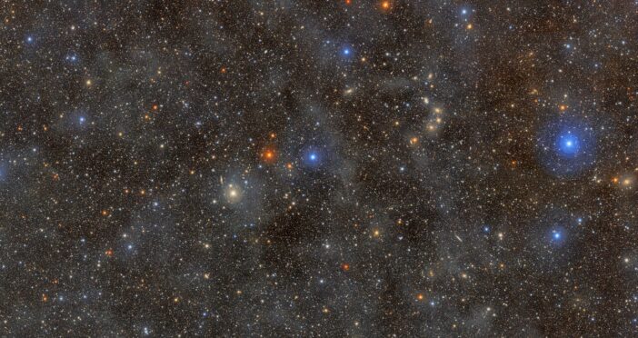
Today’s bite covers one of the NSF–DOE Vera C. Rubin Observatory‘s first major discoveries, which was found in testing data before the observatory began its decade of observations. Perched atop a mountain in Chile, the brand-new Rubin Observatory is just beginning a 10-year survey called the Legacy Survey of Space and Time (LSST). LSST will be the deepest and widest sky survey ever conducted, taking images of the entire southern night sky every three nights. This ultra-wide, ultra-high-definition time-lapse of the universe will help answer fundamental questions about dark matter and dark energy, study objects in our solar system, find distant supernova explosions, and more.

LSST is a photometric survey, meaning its main data product is images in several filters. These images are taken with the largest digital camera ever constructed, about the size of a Mini Cooper. The LSST camera has a resolution of 3.2 gigapixels. To put that number into perspective, you would need about 13 copies of the Las Vegas Sphere to display just a single LSST image… and hundreds of these images will be taken every night!

The authors of today’s article use the first dataset from the LSST camera, called Early Data Preview 2 (EDP2). EDP2 was taken from April 2025 to January 2026, covered about 3,000 square degrees (about 7% of the entire night sky), and primarily served as a test before beginning the 10-year LSST (which began in June 2026).

Small Galaxies, Big Questions

Since LSST will survey a large area at unprecedented depths, one field of interest is to study extremely dim and small galaxies called ultra-faint dwarf galaxies (UFDs). These galaxies are so faint that we can only find them close to home, orbiting the Milky Way and other nearby galaxies as satellites. UFDs don’t have much luminous matter, meaning they are likely dominated by their dark matter halos. This makes them useful test beds for our theories of dark matter and galaxy formation, if we can spot them.

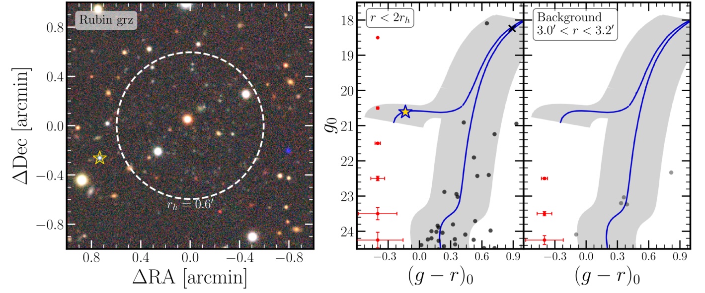
Many UFDs don’t look like normal galaxies that resemble blobs of diffuse light with stars; instead, they’re more like a handful of individual stars in an image that also contains foreground stars and background galaxies. So how do you identify them? The trick is that stars born together at the same time from the same gas follow a predictable track in color and brightness called an isochrone. The authors slide a model isochrone for an ancient, metal-poor population through the data at a range of assumed distances and ask: at any spot in EDP2, are there more stars sitting on that track than random chance would predict? Cerny and coauthors found a new spot, which they call Aquarius IV, a new UFD candidate (Figure 1).

Rubin image centered on Aquarius IV

Figure 1: Left: A Rubin image centered on Aquarius IV, combining images in the g, r, and z filters. The dashed circle marks the half-light radius, the region enclosing half the galaxy’s light. Aquarius IV is only a scattering of individual faint stars. The yellow star marks a likely blue horizontal-branch member. Right: A plot of brightness against color for the stars inside twice the half-light radius (first panel) and inside a ring of sky just outside the galaxy (second panel). Stars born at the same time from the same gas fall along the isochrone (blue line; any stars in the grey regions are deemed to follow the isochrone). All the stars follow the isochrone in the first panel but not the second, indicating that the stars are associated. [Adapted from Cerny et al. 2026]

Aquarius IV had not been identified previously by any other observatory. However, the authors combed through data from LSST’s predecessor (the Dark Energy Survey, which concluded taking data in 2019) and found previously missed evidence that supports their discovery, namely an excess of faint, blue, marginally resolved stars. As a sanity check, they confirm that all previously known UFDs within the EDP2 footprint (Sagittarius II, Aquarius II, Aquarius III, and Virgo III) are also detected using their methods.

The authors also infer several properties of Aquarius IV, including its centroid coordinates, half-light radius, ellipticity, distance, and absolute magnitude. They find that its radius is larger than almost all Milky Way globular clusters (tight gravitationally bound systems of old stars that don’t reside in their own dark matter halos), suggesting that Aquarius IV is a true dwarf galaxy.

Currently, there are about 40 known UFDs around the Milky Way, and LSST is expected to roughly double this number (see this Astrobite), allowing us to study these tiny galaxies at a population level. This article proves that LSST has the potential to revolutionize many areas of astrophysics! If you are a researcher in the US or Chile and want to play with the EDP2 data yourself, you can access it via the Rubin Science Platform. For researchers from other countries, see more info here.

Original astrobite edited by Katya Gozman.

About the author, Ben Sherwin:

I am a physics PhD student and NSF Graduate Research Fellow at Stanford University. I am interested in theoretical and observational cosmology, specifically in cross-correlations between the cosmic microwave background and tracers of large-scale structure. Outside of work, I enjoy seeing the latest movies in theaters and exploring the San Francisco Bay Area.

The post An Early Discovery by Rubin Observatory appeared first on AAS Nova.

  •  

A Sneak Peek into Early-Universe Star Formation with Boötes I

star-forming region N44

Editor’s Note: Astrobites is a graduate-student-run organization that digests astrophysical literature for undergraduate students. As part of the partnership between the AAS and astrobites, we occasionally repost astrobites content here at AAS Nova. We hope you enjoy this post from astrobites; the original can be viewed at astrobites.org.

Title: Probing the IMF in the Early Universe — Direct Measurements in the Boötes I UFD with JWST/NIRCam
Authors: Keyi Ding et al.
First Author’s Institution: University of Maryland
Status: Published in ApJ

The Stellar Initial Mass Function

plot of different formulations of the initial mass function

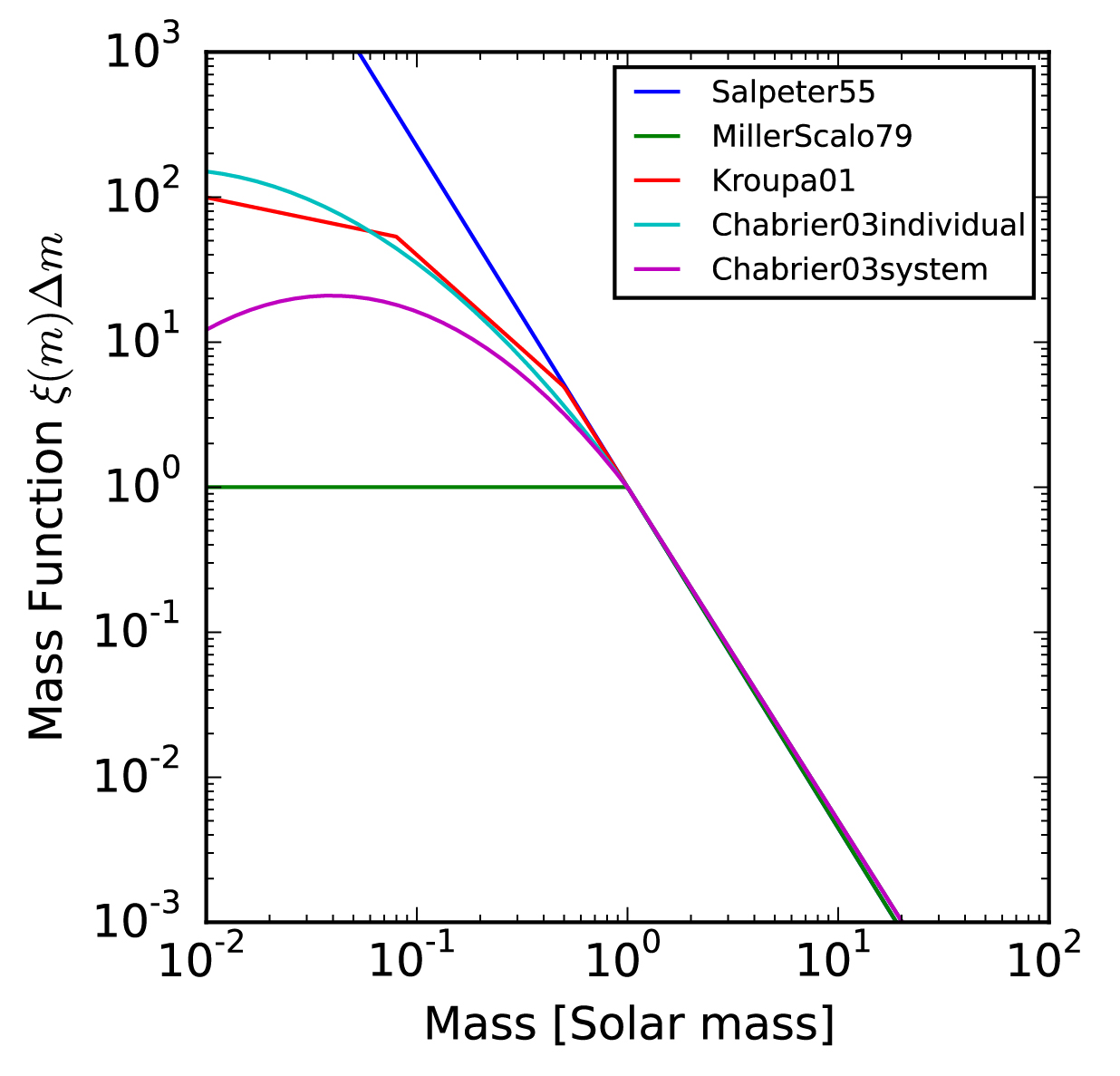
Figure 1: Several different formulations for the IMF. Astronomers have found that the Milky Way IMF seems to follow either a broken power law (Kroupa), or a log-normal (Chabrier) distribution. [JohannesBuchner; CC BY-SA 4.0]

A fundamental concept in astronomy is the stellar initial mass function (IMF). The IMF describes the number of stars of each mass that form from a single birth cloud. If the IMF has a negative slope, it means most stars are low in mass; if it has a positive slope, it means most stars are high in mass. Figure 1 shows some examples of commonly used IMFs, all of which have a negative slope, since we see far more low-mass stars than high-mass stars in the Milky Way. You may notice that several models deviate from a straight line at about 0.5 solar mass. This point, known as the turnover or critical mass, is crucial in determining the exact shape of the IMF.

For a relatively simple concept, the IMF is shaped by incredibly complicated underlying physical mechanisms. Things like turbulence, magnetic fields, and chemical enrichment all play a role in shaping the observed IMF. Additionally, the IMF is a pretty fundamental quantity. An enormous amount of astronomy research relies on assumptions made about the IMF. For example, since most stars are low in mass, and low-mass stars are dimmer, astronomers use the IMF to convert the amount of light in a galaxy to the number of stars; if there are more or fewer low-mass stars than we expect, our measurements will be wrong.

A big question surrounding the IMF is whether or not it’s universal. In the Milky Way, astronomers have been able to measure the IMF accurately, and they have found that it seems to be the same regardless of which bunch of stars we use to measure it.1 However, we know that galaxies in the early universe were very different compared to today. Things get tricky when you acknowledge that most measurements made of early-universe galaxies rely on modeling tools that are entirely reliant on assuming an IMF. This gnarly little detail makes measuring the IMF in the early universe especially valuable to astronomers.

What Makes Ultra-Faint Dwarfs So Special?

Today’s authors attempt to measure the early-universe IMF using a local relic, an ultra-faint dwarf galaxy (UFD). You might describe UFDs as “incredibly funky little galaxies.” They’re much less massive than the Milky Way, with about 10,000 times less stellar mass. What stars they do have tend to be very old and metal poor. The nature of UFDs has led many astronomers to think of them as fossils: relatively untouched galaxies formed in the early universe. Since we think UFDs are fossils of earlier galaxies, measuring the IMF in a UFD tells us whether the IMF was the same in the early universe as it is today. The authors focus on Boötes I, a relatively luminous UFD orbiting the Milky Way. Figure 2 shows Boötes I as seen by the Sloan Digital Sky Survey.

Boötes I

Figure 2: Boötes I as seen by the Sloan Digital Sky Survey. Because they’re so diffuse, UFDs look less like galaxies and more like groups of stars. [Vasily Belokurov – SDSS-II Collaboration]

The IMF in Boötes I

Measuring the IMF can get tricky — it’s typically pretty difficult to measure the mass of each individual star in a galaxy. Thankfully, Boötes I is close enough that we can do exactly that! Using JWST’s NIRCam instrument, today’s authors obtain imaging of Boötes I that is sensitive enough to extract roughly 10,000 stars belonging to the galaxy.

To measure the IMF from the observed population of stars, the authors use a modified version of Starwave, a Bayesian inference tool. In short, the tool takes in some assumptions about the population of stars in the galaxy, then generates many potential color–magnitude diagrams for various parameter selections. You can then assess how well each simulated color–magnitude diagram fits the observed data, thus determining likely parameters for the stellar population. The authors apply their tool for three different IMF models, testing how close the IMF in Boötes I is to that of the Milky Way. This allows them to determine how well the IMF compares to that of the Milky Way, which is typically thought of as a broken power law or log-normal distribution. If the IMF in Boötes I aligns with the Milky Way’s IMF, we’ll have a solid piece of evidence for a truly invariant IMF across cosmic time, allowing astronomers to rest easy knowing our modeling efforts haven’t been bunk this whole time.

So… What Did We Learn?

The authors find that a single power law can be ruled out to a good degree of confidence. This is good, as Milky Way studies show undeniable evidence of a turnover in the distribution. The broken power law and log-normal models both fit the observed data relatively well, aligning well with Milky Way–derived IMFs. All in all, they find solid evidence for an invariant IMF in the early universe.

However, they are unable to say with absolute certainty that the IMF is invariant. Given that their data are nearly perfect (that is, it’s pretty much impossible to get better data for Boötes I), the authors emphasize that a larger sample of UFD IMFs is needed to truly rule out an invariant IMF, but we’re certainly taking steps in the right direction! As the age-old saying goes, “more data are needed!”

Original astrobite edited by Maggie Verrico.

  1. Editor’s Note: The Milky Way IMF may vary from star cluster to star cluster; as described in this AAS Nova highlight from 8 July 2026, recent research using data from the Gaia spacecraft has found evidence for IMF variation in our galaxy. ↩︎

About the author, Drew Lapeer:

Drew is a first-year PhD student at the University of Massachusetts Amherst. They are broadly interested in the evolution of galaxies, with a focus on the impact of cosmic feedback on the galactic ecosystem. In their free time, they enjoy reading, rock climbing, hiking, and baking!

The post A Sneak Peek into Early-Universe Star Formation with Boötes I appeared first on AAS Nova.

  •  
❌